Penalised spline regression

Sometimes you don’t know the functional form of a regression relationship. In such an instance, the use of a penalised spline regression can help you model it without having a ridiculously wiggly smooth function.

Motivation

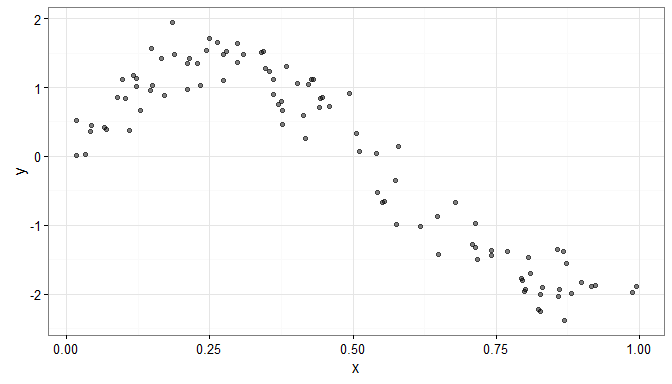
Consider some simulated data for which it is not obvious what the functional form of the relationship is.

N <- 100
x <- sort(runif(n=N, min = 0, max = 1))
y <- sin(2*pi*x) - 5*x^2 + 3*x + rnorm(n=N, sd=0.25)

dat <- data.frame(y=y, x=x)

library(ggplot2)
gg.data <- ggplot(data=dat, aes(x=x, y=y)) +
  geom_point( alpha=0.5) + theme_bw()

Splines

In order to model the effect of x on y we may wish to fit a regression model. If we aren’t explicitly interested writing down a parametric equation, we can use a spline to flexibly model this relationship (Eilers and Marx 2010).

The choice of what kind of spline to use and how many basis splines can be important. Too many basis splines and we end up with a fitted smooth that is very wiggly; too few and we may not be able to capture the variability.

B-splines

• The B-spline is a common choice for producing smooth functions (de Boor 1977)
• The P-spline (Eilers and Marx 1996) penalises changes in the second derivative of the B-spline
• Ruppert, Wand, and Carroll (2003) discuss choice of knots
• Lang and Brezger (2004) formulated this in a Bayesian framework
• Rue and Held (2005) discuss this as an intrinsic CAR prior

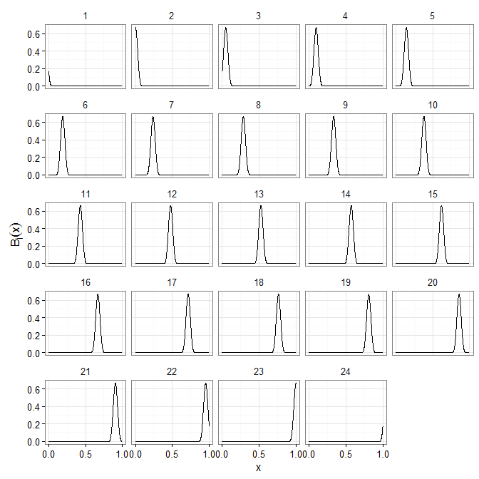
The basis matrix

The basis matrix is calculated according to the formulation given by Eilers and Marx (1996). Here we choose a number of basis splines given by the advice in section 3 of Wand (2000).

d <- max(4, floor(N/35))
K <- floor(N/d - 1)

bspline <- function(x, K, bdeg=3, cyclic=FALSE, xl=min(x), xr=max(x)){
  x <- as.matrix(x,ncol=1)
  
  ndx <- K - bdeg
  
  # as outlined in Eilers and Marx (1996)
  dx <- (xr - xl) / ndx
  t <- xl + dx * (-bdeg:(ndx+bdeg))
  T <- (0 * x + 1) %*% t
  X <- x %*% (0 * t + 1)
  P <- (X - T) / dx
  B <- (T <= X) & (X < (T + dx))
  r <- c(2:length(t), 1)
  
  for (k in 1:bdeg){
    B <- (P * B + (k + 1 - P) * B[ ,r]) / k; 
  }
  
  B <- B[,1:(ndx+bdeg)]
  
  if (cyclic == 1){
    for (i in 1:bdeg){
      B[ ,i] <- B[ ,i] + B[ ,K-bdeg+i]    
    }
    B <- B[ , 1:(K-bdeg)]
  }
  
  return(B)
}



X <- bspline(x, K, xl=0, xr=1)

We also want to predict, so need to re-use the same number of knots and endpoints from the original spline to set up a prediction matrix.

x.pred <- seq(0, 1, length.out=1001)

X.pred <- bspline(x.pred, K, xl=0, xr=1)

What does our basis look like?

Formulating penalty matrix

For a B-spline with K basis splines, we need to differentiate a K × K identity matrix a number of times equal to the order of the penalty

We add a small value to the diagonal to ensure the matrix is symmetric, positive, definite

• we know the matrix is symmetric
• we need eigenvalues real and greater than 0

makeQ = function(degree, K, epsilon=1e-3){
  x <- diag(K)
  E <- diff(x, differences=degree)
  return( t(E) %*% E + x*epsilon)
} 

Q <- makeQ(2, K)

Without the small amount on the diagonal

round(eigen(makeQ(2, K))$values, 5)
##  [1] 15.85603 15.42770 14.73537 13.80996 12.69206 11.42942 10.07411
##  [8]  8.67940  7.29673  5.97289  4.74756  3.65150  2.70540  1.91948
## [15]  1.29383  0.81951  0.48020  0.25428  0.11730  0.04434  0.01241
## [22]  0.00251  0.00100  0.00100

round(eigen(makeQ(2, K, epsilon=0))$values, 5)
##  [1] 15.85503 15.42670 14.73437 13.80896 12.69106 11.42842 10.07311
##  [8]  8.67840  7.29573  5.97189  4.74656  3.65050  2.70440  1.91848
## [15]  1.29283  0.81851  0.47920  0.25328  0.11630  0.04334  0.01141
## [22]  0.00151  0.00000  0.00000

we see eigenvalues of 0 (or close to) which leads to, at best, and ill-conditioned system or, at worst, a degenerate precision matrix that can’t be factorised

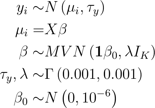
Fitting the model

For our simple univariate spline, we fit the model

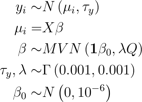
The following model code was used in JAGS to fit the above model:

model{
  for (i in 1:n){
    y[i] ~ dnorm(mu[i], tau.y)
    mu[i] = X[i, ] %*% beta[1:K]
  }
  
  beta[1:K] ~ dmnorm(beta.0[1:K,1] + beta.00, lambda*Q[1:K,1:K])
  
  gamma <- beta - beta.00
  
  tau.y ~ dgamma(0.001, 0.001)
  lambda ~ dgamma(0.001, 0.001)
  
  beta.00 ~ dnorm(0, 1e-6)

  for (j in 1:m){
    y.rep[j] ~ dnorm(mu.rep[j], tau.y)
    mu.rep[j] = X.pred[j, ] %*% gamma[1:K] + beta.00
  }
}

Results

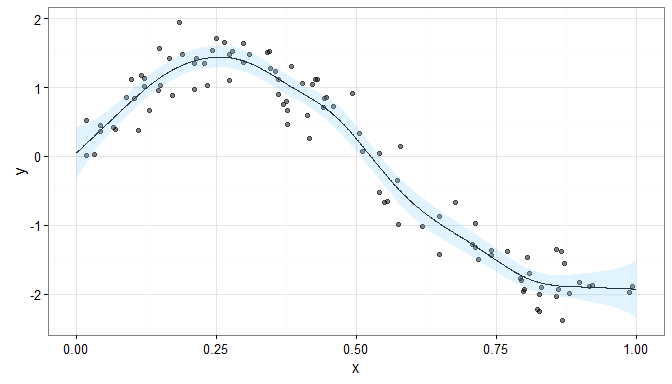
If we didn’t penalise our spline, we would have the model

where I_K is the K × K identity matrix, and the resulting smooth would look like

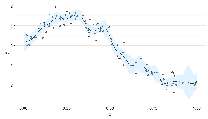
This fitted smooth is much more wiggly than the penalised smooth

Conclusion

B-splines are great for non-linear relationships without strict a priori assumptions about the functional form.

Penalisation smooths your smooths even further

• not as susceptible to local changes
• posterior distribution of λ informed by data, not fixed and cross-validated as in Frequentist penalised likelihood smoothing

References

de Boor, Carl. 1977. “Package for Calculating with B-Splines.” SIAM Journal on Numerical Analysis 14: 441–72.

Eilers, Paul H. C., and Brian D. Marx. 1996. “Flexible Smoothing with B-Splines and Penalties.” Statistical Science 11: 89–121.

———. 2010. “Splines, Knots and Penalties.” Wiley Interdisciplinary Reviews: Computational Statistics 2: 637–53. doi:10.1002/wics.125.

Lang, Stefan, and Andreas Brezger. 2004. “Bayesian P-Splines.” Journal of Computational and Graphical Statistics 13 (1): 183–212.

Rue, Havard, and Leonhard Held. 2005. Gaussian Markov Random Fields: Theory and Applications. CRC Press.

Ruppert, David, Matt P. Wand, and Raymond J. Carroll. 2003. Semiparametric Regression. Cambridge University Press.

Wand, Matt P. 2000. “A Comparison of Regression Spline Smoothing Procedures.” Computational Statistics 15: 443–62.