Changes in character time series
27 Jan 2016 | web: Sam Clifford | github: samcliffordtags: r, dplyr, ggplot2 |

Description
Sometimes in time series you have a set of states for which you may spend a certain amount of time before switching to another state or returning to a previous one (e.g. whether a student is indoors at school, outdoors at school, commuting, indoors at home, etc.).
A straight up factor to numeric conversion won’t work, because we want to assume that returning to a previous value.
library(ggplot2)
library(dplyr)
First we’re going to simulate some data that behaves the way we discussed above.
N <- 10

labels <- letters[sample(x = 1:4, size = N, replace = T)]

n.each <- rpois(n=N, lambda=40)

my.x <- data.frame(label=rep(labels, times=n.each),
                   x = 1:sum(n.each),
                   y = rnorm(n=sum(n.each)))

ggplot(data=my.x, aes(x=x, y=y)) + geom_line(aes(color=label)) + theme(legend.position="bottom")
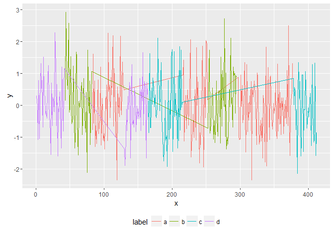
Obviously the grouping by the variable type here not only looks strange in ggplot2 but we don’t have an ID for unique instances of each label.
We will turn the input variable into a numeric vector and then look at where it changes. Loop over the endpoints and sequentially increase a counter index between the endpoints.
detect_text_changes <- function(x){
  x1 <- as.numeric(factor(x))

  diff1 <- diff(x1)

  changes <- c(0, which(diff1 != 0), length(x))

  values <- rep(NA, length(x))

  for (i in 2:length(changes)){
    values[(changes[i-1]+1):(changes[i])] <- i-1
  }

  return(values)
}

my.x <- mutate(my.x, label.new = detect_text_changes(label))
Let’s plot with our new labelling scheme
ggplot(data=my.x, aes(x=x, y=y)) + geom_line(aes(color=label, group=label.new)) + theme(legend.position="bottom")
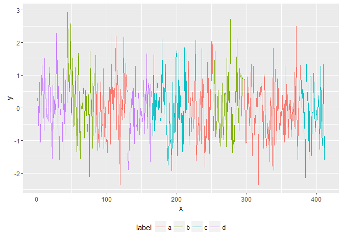
We can now summarise either by label without distinguising between unique instances or summarise by instance.
my.x %>% group_by(label) %>% summarise(mean = mean(y))
## Source: local data frame [4 x 2]
##
##    label        mean
##   (fctr)       (dbl)
## 1      a -0.01950181
## 2      b  0.15706226
## 3      c -0.06210777
## 4      d  0.01293803
my.x %>% group_by(label.new, label) %>% summarise(mean = mean(y)) %>% arrange(label.new)
## Source: local data frame [9 x 3]
## Groups: label.new [9]
##
##   label.new  label         mean
##       (dbl) (fctr)        (dbl)
## 1         1      d  0.108663695
## 2         2      b  0.198499260
## 3         3      a  0.046210382
## 4         4      d -0.101932775
## 5         5      c -0.004878618
## 6         6      a  0.022771377
## 7         7      b  0.118516222
## 8         8      a -0.076240612
## 9         9      c -0.145498828